Luminosity Fitting, Lambda Fitting, SNLS data and minimum error calculation

The SuperNovea Legacy Survey project is involved with measuring magnitudes of Super Novae type 1A.
Luminosity Fitting is the methode used in order to fit observation data collected by SNLS project with the theoretical data using Friedmann's equation.

• The SNLS data shows the relation between magnitude and z. See: Figure 11.
• The calculations of the Friedmann equation show the relation between distance and z

In order to calulate magtitude from distance (or reverse) you need the following three equations:

1. F = L/(4*pi*d*d) This is called FL relation 1. L is called Luminosity. F is called Flux.
2. K = 10 Log(F) :
3. m = -2.5*K+n with n=0. m = magnitude

FL relation 1 shows the relation between Flux versus L (Luminosity) as a function of distance. Different FL relations are possible. For an overview of FL relations go to: Friedmann's Equation Question 7

Luminosity Fitting

This involves to calculate the Luminosity (L) parameter which closest matches the SNLS data. In order to do that you have to calculate error values (See next paragraph) as a function of z values of SNLS data and friedmann's equation.
One error values as a function of L is calculated as follows:

1. You start from the SNLS data. The magnitude axis which runs between 13 and 26 is divided in 52 segments equal segements.
2. For each of those segments is the z value is calculated and stored in the array z1(n).
3. Next the Friedmann equation is used. Friedmann's Equation The result are stored in two arrays dist(i) and z(i) with i values as a function of C, Lambda and k.
4. Using the above 3 equations for each dist(i) the magnitude parameter m is calculated as a function of L and stored in an array magn(i).
5. Next using z(i) and magn(i) for the same 52 segments as for the SNLS data z values are calculated and stored in the array z2(n)
6. The difference between the 52 z1 and z2 values is calculated and squared.
7. The sum of all the squared n=52 segments is calculated.
8. Finally from that number the root is taken and divided by n=52. The result is the error value

Luminosity Fitting starts with 4 different estimates of L.

For example 0.0000001, 0.0000002 0.0000003 and 0.0000004

Next for each of those values an error values is calculated as explained above.

Suppose the 4 error values are 10, 7, 6 and 11

The first L value is definite not the smallest. That one drops off.
The new 4 L values are: 0.0000002 0.0000003 0.00000035 and 0.0000004.
#3 is new and an error value is calculated.

Suppose the 4 error values are 7, 6, 8 and 11

The last L value is definite not the smallest. That one drops off.
The new 4 L values are: 0.0000002 0.00000025 0.0000003 and 0.00000035. #2 is new calculated.

Suppose the 4 error values are 7, 5.5, 6 and 8

This whole process is repeated 25 times
The result is the optimum Luminosity value which closest matches the SNLS data

Error value calculation

The error value of an array a(n) compared with an array b(n) of both 52 values is calculated as:

1. Error_sum = (a(n) - b(n)) ^ 2 with n going from 0 to 52.
2. Error = Square root(Error_sum) / 52

Lambda Fitting

Lambda Fitting is almost the same as Luminosity Fitting. The objective is to find the Lambda value for a certain FL relation

1. We start with 4 different Lambda values.
   
   For example 0.01 0.02 0.03 and 0.04

   For each of those values Luminosity Fitting is performed. The result is 4 error values

   For example: 4.1 3.5 3 and 3.9

   The first Lambda value is definite not the smallest and is dropped.

   The 4 different Lambda values are: 0.02 0.03 0.035 and 0.04.

   Luminosity Fitting is performed for value #3.

   The result is 4 error values 3.5 3 3.6 and 3.9

   The fourth Lambda value is definite not the smallest and is dropped.

   The 4 different Lambda values are: 0.02 0.025 0.03 and 0.035

   Luminosity Fitting is performed for value #2.

   The result is 4 error values 3.5 3.1 3 and 3.6

   This whole process is repeated 25 times.
   The result is the optimum Lambda value which closest matches the SNLS data.

Care should be taken in case error value 4 is the smallest. In that case a value outside the range should be tried.

• For example if the Lambda values are : 0.01 0.02 0.03 and 0.04 and the error values are 4 3 2 and 1
  Than the new Lambda values are: 0.02 0.03 0.04 and 0.05
  
• If the new error values are (with Luminosity Fitting #4 calculated) : 3 2 1 and 1.5
  Than you can proceed as explained previous.

Following are three figures with explain the above information.

1. Figure 1 is used to demonstrate the magnitude versus Z relation for the same Friedmann equation. The parameter Lambda = 0.02049 in each case is the same.

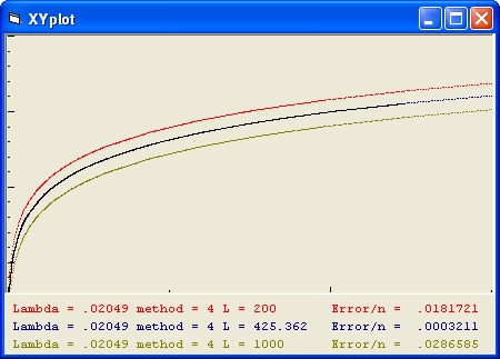   Figure 1 Magtitude versus Z

   The black line shows the SNLS data
   The blue line shows the condition with Luminosity Fitting
   The Lambda value of the blue line is calculated by using Lambda Fitting.
2. Figure 2 is used to demonstrate the magnitude versus z relation for the 3 different Friedmann equations. The parameter Lambda is different in each case. The Luminosity parameter L is the same.

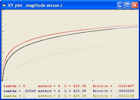   Figure 2 Magtitude versus Z

3. Figure 3 demonstrates the same Lambda values as in figure 2. The difference is that Luminosity Fitting is used for the red and yellow line.

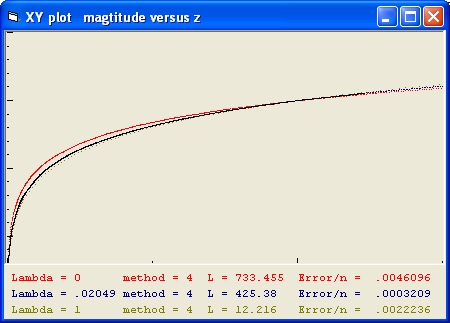   Figure 3 Magtitude versus Z

Back to Friedmann's equation: Friedmann's Equation & The path of a light ray FL relation #1
Back to my home page Contents of This Document